Lab 4: Special Signals TIMS

Table of Contents

1 Introduction
2 Procedures
3 Conclusion

1 Introduction

This lavatory introduces how to using the clock signal to synchronize and reference the output signal transformed by various signal processing effects.

2 Procedures

2.1 The Audio Oscillator

This part shows how to used the square wave generated by Audio Oscillator, measuring the clock rate by Frequency Counter, and using PicoScope to measure the pulse width.

The measured pulse width is $407.3 μ s$ and the clock cycle is $1000.2 μ s$ .

2.2 The Sequence Generator

This part shows how to used the clock signal provided by Audio Oscillator to generate a random bit stream with Sequence Generator.

The minimum interval of the digital signal is measured as $995.9 μ s$ , which is about the same of the clock cycle duration.

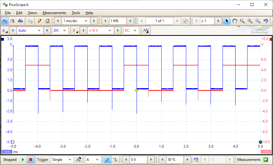
In Figure 2.2.1, Comparing clock signal and generated random sequence, the binary code corresponding to the digital signal is 100010101....

The square clock signal and random bit stream

Figure 2.2.1 Comparing clock signal and generated random sequence

2.3 Baseband Channel Filter

The Baseband Channel Filter provides three different filters. This part shows how to measure the transition time of the output signal produced by the filter.

Table 2.3.1 Delay and Transition Times for Sequence Data (at 1kHz)

time(ms)	BBLPF2	BBLPF3	BBLPF4
Delay	0.24	0.25	0.84
Rise	0.71	0.29	0.18
Fall	0.23	0.31	0.19

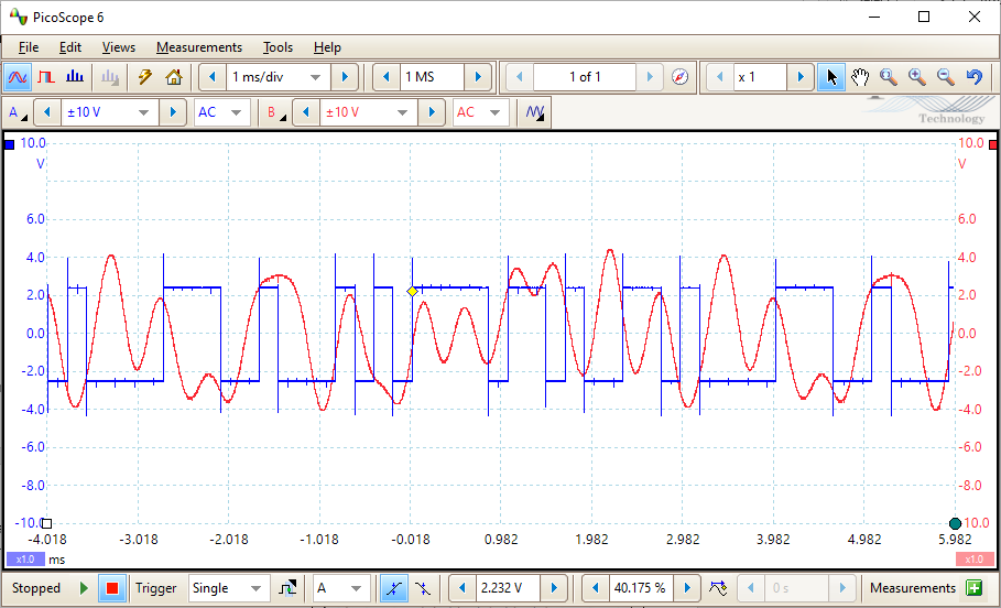
The next part of the experiment shows how increasing the frequency of the input affects the distortion of the output signal. Figure 2.3.1, Comparing the input clock with output of low-pass filter shows at about 4.7kHz it is unable to discern the original digital signal from output of BBLPF4.

The square clock signal and the filtered result

Figure 2.3.1 Comparing the input clock with output of low-pass filter

2.4 Step Input

This part shows the technique known about Step Input to measure the delay time and rise time of the filtered signal. This is essentially about using a step function to check the response signal.

Table 2.4.1 Step Response for Various Filter Systems (low f setting)

time(ms)	BBLPF2	BBLPF3	BBLPF4
Delay	0.22	0.27	0.82
Rise	0.23	0.27	0.20

2.5 Impulse

This part approximates the impulse function by using the SYNC signal provided by Sequence Generator.

According to Table 2.5.1, Pulse Width Data, when the frequency increase, the pulse width decreases.

The amplitude of filtered signal decreases as pulse width reduces, since there are less time from the response signal to increase.

Table 2.5.1 Pulse Width Data

f (cycles per second)	Pulse Width (us)
500	1986
1000	996.9
1500	666.5
2000	497.7
3000	331.8
4000	249.7
6000	167.0
8000	124.8
10000	100.1

An inverse proportion relation between frequency and pulse width.

Figure 2.5.1 Plot of Pulse Width Data

2.6 Basic Sine Waves

This part measures the affect of low-pass filter one sine wave of different frequencies. In Table 2.6.1, Amplitude at different input frequencies, the signal quality drops as the frequency gets higher, which makes the result harder to measure.

Table 2.6.1 Amplitude at different input frequencies

Frequency	BBLPF2	BBLPF3	BBLPF4
Hz	Vpp	Vpp	Vpp
300	6.602	6.427	6.733
1000	6.252	4.853	6.701
2000	4.678	2.077	5.684
3000	0.481	0.445	0.612
4000	0.074	0.084	0.082
5000	0.029	0.034	0.056

2.7 Clipping

The step 1-5 in this part demonstrates the Utilities module and its Clipper. The peek of the sine wave has been flatten during the clipping. When the signal amplified to 20Vpp, the output signal has become a almost exact square wave.

2.8 Digital Detector

The digital detector can be used to restore a distorted digital signal. In Table 2.8.1, Comparing recovered digital signal to original digital signal, it can be seen that the restore signal is inverted, and at higher frequency rate it is much harder to restore the signal.

Table 2.8.1 Comparing recovered digital signal to original digital signal

f (kHz)	Input digital signal	Output digital signal
4	10100001	0101110
5	11001011	00110100
7	00101111	00110000

3 Conclusion

In this laboratory experiment, the components we used to build the signal are not very complex and it is easy to guess how each components could be implemented by examine the circuit, which is where I enjoy about this lab.

The PicoScope can add measurement to track Vpp which can make measurement in Table 2.6.1, Amplitude at different input frequencies tremendously easier.

I think the Fig 29 of the instruction sheet is wrong, as the Audio Oscillator sin output is plugged to the digital input of Frequency Counter rather than the analogue input, which would not give the expected result shown in Fig 30(a).