1 Introduction
This exercise demonstrates how to define and organize functions in MATLAB. We would define a few commonly find signal functions and make plots of them using MATLAB.
2 Procedure
2.1 Write a MATLAB function
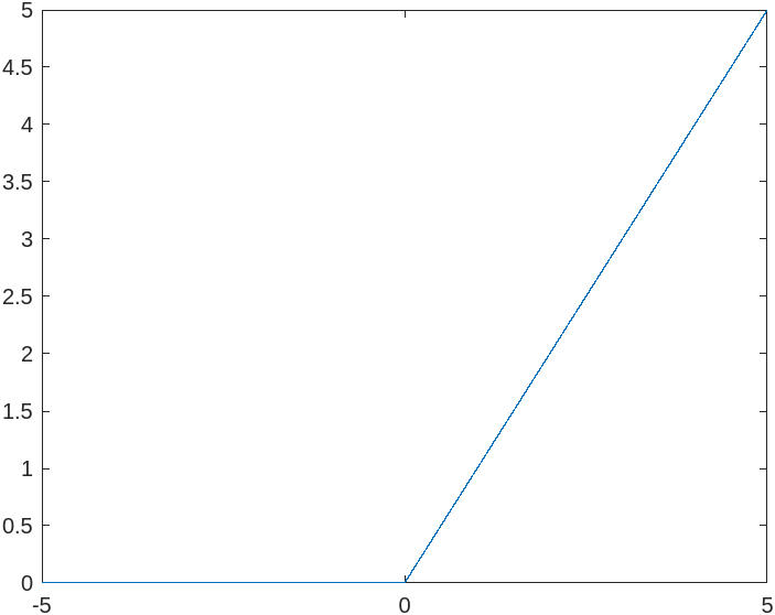
The statements below plots the step function by feeding an array
from -5 to 5 to the function.
>> t = -5:0.001:5;
>> plot(t,u(t,0))
If step size is changed from 0.001
to 0.1, the resolution, or sample
rate, would be lowered. In this case a small ramp is created
near t=0 due to the lowered
resolution.
The statement y=t>=to in u(t,to) compares a numeric array to a scalar and
return the result as an array of 0 or 1s, and assign the result to
the variable y.
2.2 Ramp function
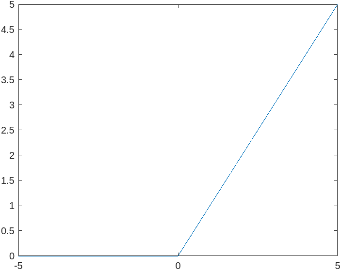
The statement y=(t-to).*(t>=to) sets
y to the element-wise multiplication
of the two arrays t-to and
t>=to.
Setting t=-5:0.001:5 and t=-5:1:5 then
do plot(t,r(t,0)) respectively. Figure 2.2.1, Ramp plot at step
size 0.001 uses the step size 0.001 while Figure 2.2.2, Ramp plot at step size 1 uses step
size 1.
2.3 Plotting skills
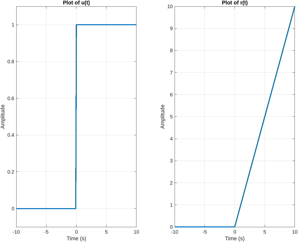
|clc|clear|close all|t=-10:0.1:10;5 |y_u=u(t,0);|y_r=r(t,0);|subplot(1,2,1);|plot(t,y_u,'LineWidth',2)|title('Plot of u(t)')10 |xlabel('Time (s)')|ylabel('Amplitude')|ylim([-0.1 1.1])|grid on|subplot(1,2,2);15 |plot(t,y_r,'LineWidth',2)|title('Plot of r(t)')|xlabel('Time (s)')|ylabel('Amplitude')|grid on
This creates Figure 2.3.1, Unit step and ramp.
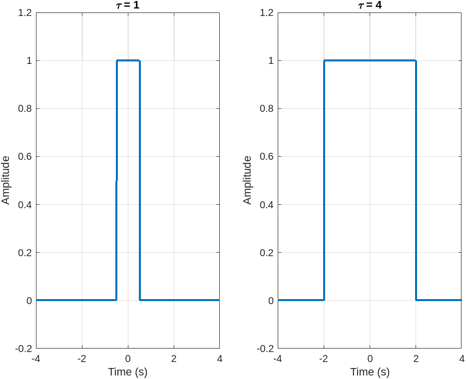
2.4 Build the Pulse function
|function y = p(t,tau)|% p(t,tau) defines the pulse function|y=((-tau/2)<=t).*(t<=(tau/2));|end
2.5 Generate a script with different sections


3 Feedback
The function syntax used in MATLAB resembles APL a lot:
  |∇y←u (t to)
  | y←t≥to
  |∇
Since I'm using the web version of MATLAB, the resulted plotting has been out of proportion a bit.
Besides, I think it is worth pointing out that MATLAB automatically interpret label text as LaTeX, and it would be helpful to give a feel samples on how to write equations in LaTeX for students who had on prior experience.