1 Introduction
This exercise demonstrates using MATLAB to solve for the transfer function of a complex circuit. A circuit is transformed to Laplace domain and solved for the impulse response, and various tools are used to simplify and visualize the transfer function.
2 Procedure
2.1 Transform circuit to Laplace Domain
First of all, connecting the ground node of the input to the
ground node of R6, which would become
the mesh for I3.
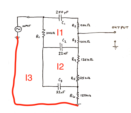
The mesh analysis on the circuit transformed to Laplace domain give the matrix:
2.2 Derive the expression for output voltage
The expression of output voltage is the sum of voltage across
R3, R4,
R5 and R6.
The numden function is used to
extract the numerator and denominator.
2.3 Simplify the expression
We would first convert the numerator and denominator polynomial to array, and divide them by a common factor.
The result would cause the first few coefficients to be displayed as zero, due to it is very small so the display routine rounded it. The value is still preserved in the result array, however.
2.4 Plot the result
The plotted result is in Figure 2.4.1, Plot of BODE, step function, and poles.
The BODE plot shows if the input is a sine wave, how the change of input frequency affects the output magnitude and the phase shift.

3 Feedback
This lab shows how to decompose tedious manual computations into programs, which a few hints on how to simplify the result.
It is initially a bit confusing on which three meshes to be used to setup the matrix until I read the expression for output voltage and the hint on connecting ground nodes in the circuit.
I think a brief notes on that the matrix can be setup fairly easily by counting total impedance in a current mesh and the intersection between two meshes would be very helpful.