1. Introduction
This is where we start to get used to the equipment. We will use the function generator to produce a modulated sine wave and monitor the signal on the oscilloscope. Amplitude modulation would be demonstrated.
2. Simple Sine Waves
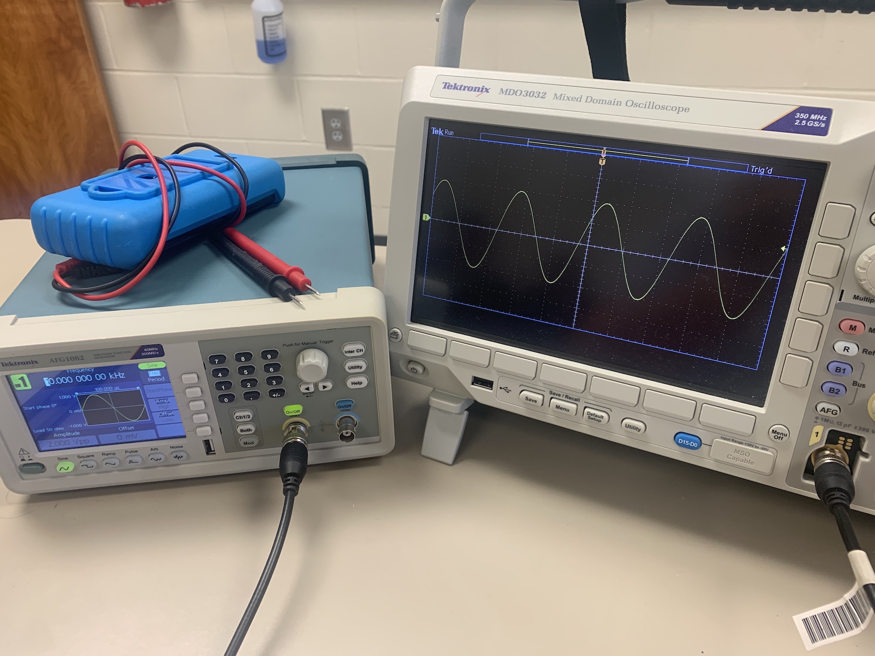
Using the AFG 1602 function generator to produce a 2Vpp 10kHz sine wave, and using a BNC-to-BNC cable to connect the function generator output to the oscilloscope's channel 1.
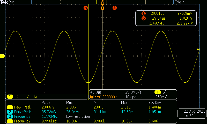
As we can see in Figure 2 the channel 1 has peak-to-peak voltage 2.008V and frequency at 9.998kHz, which matches the parameter used by the FGEN.
For the 10kHz signal, the appropriate time scale would be 50μs, and the closest scale on this oscilloscope model is 40μs.
The digital multi-meter gives a reading of 0.75V on the FGEN output, which appears to be RMS voltage.
3. Amplitude Modulation
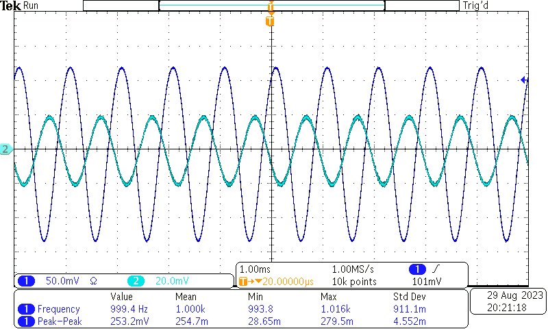
We would use a 10kHz carrier modulated bu 1kHz sine wave intelligence signal, at 50% depth modulation. Since we want to view the intelligence signal, the timescale is set to 400μs.

As we can see in the channel 1 has peak-to-peak voltage 2.008V and frequency at 9.998kHz, which matches the parameter used by the FGEN.
For the 10kHz signal, the appropriate time scale would be 50μs, and the closest scale on this oscilloscope model is 40μs.
The digital multi-meter gives a reading of 0.75V on the FGEN output, which appears to be RMS voltage.
4. AM Frequency Spectrum
For this part we use a carrier frequency of 1230kHz with amplitude 100mVpp, setting up intelligence to be 1kHz at 50% modulation.
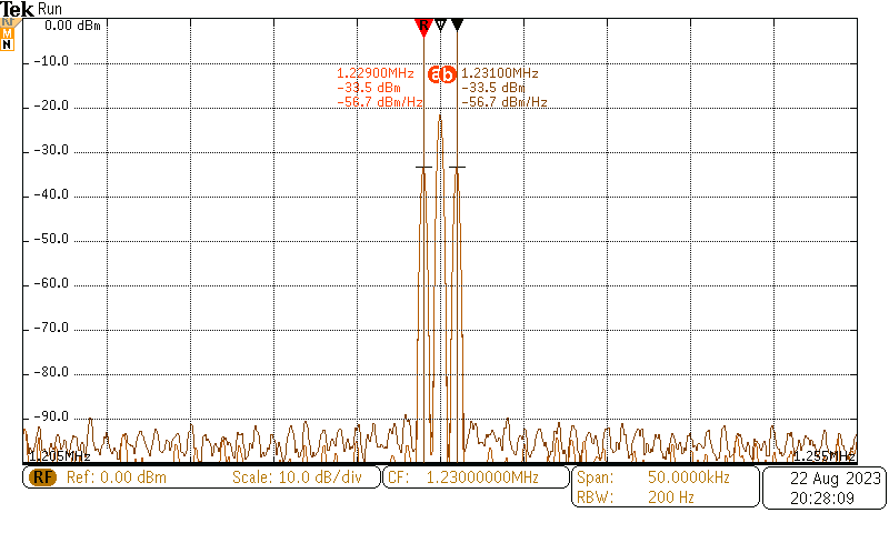
| Type | Frequency (MHz) | dBm level | Voltage amplitude (mV) |
| Lower sideband | 1.229 | -33.5 | 6.683 |
| Carrier | 1.23 | -21.5 | 26.607 |
| Upper sideband | 1.231 | -33.5 | 6.683 |
| Type | Frequency (MHz) | dBm level | Voltage amplitude (mV) |
| Lower sideband | 1.229 | -27.5 | 13.335 |
| Carrier | 1.23 | -21.4 | 26.915 |
| Upper sideband | 1.231 | -27.5 | 13.335 |
Notice that as the modulation increases, the sideband amplitude is getting higher.
Other than analyze modulated signals, the spectrum view is also good at analyzing noise and distortions.
5. AM Frequency Spectrum (FFT Method)
For this part we set carrier frequency to 50kHz with amplitude 100mVpp, setting up intelligence to be 1kHz at 50% modulation.
| Type | Frequency (kHz) | dB level | Voltage amplitude (mV) |
| Lower sideband | 49 | -44.55 | 8.376 |
| Carrier | 50 | -29.68 | 46.4 |
| Upper sideband | 1.231 | -44.59 | 8.337 |
| Type | Frequency (kHz) | dB level | Voltage amplitude (mV) |
| Lower sideband | 49 | -38.55 | 16.711 |
| Carrier | 50 | -29.66 | 46.507 |
| Upper sideband | 1.231 | -38.6 | 16.616 |
Notice that the result gain is different from the spectrum mode.
6. Conclusion
In this lab we learned how to use the function generator and oscilloscope, focused on introduction AM and how to analyze the signal from spectrum view.
7. Introduction
In this lab we will learn how to build a CE amplifier circuit measure the bandwidth/gain of it.
8. The DC measurement
After building the DC circuit of the amplifier, it is a good ideal to measure the voltage to determine if these matches the simulated bias point.
My measured VBE is 0.71V, VCE is 4.36V which is greater than 0.2V, indication the BJT transistor is in forward active mode.
| Node | Measured | Simulated |
| VB | 1.83 | 1.875 |
| VC | 5.48 | 5.357 |
| VE | 1.12 | 1.166 |
9. Amplifier gain
| RL(Ω) | Voltage Gain |
| 10 | 2.62 |
| 100 | 9.075 |
| 1k | 12.74 |
| 10k | 12.74 |
| 100k | 13.665 |

This indicates that for an 8Ω speaker the CE amp could only provide less than 2.6V/V gain.
| Frequency (Hz) | Voltage Gain | Gain (dB) |
| 100 | 1.025 | 0.214 |
| 300 | 6.01 | 15.577 |
| 1k | 12.75 | 22.11 |
| 3k | 15.62 | 23.87 |
| 10k | 15.90 | 24.03 |
| 30k | 16.01 | 24.09 |
| 100k | 16.51 | 24.35 |
| 300k | 16.63 | 24.42 |
| 1M | 16.75 | 24.47 |
| 3M | 16.45 | 24.32 |
| 10M | 12.42 | 21.88 |

From Figure 7 we can observe the 3dB bandwidth is from 1kHz to 1.4MHz.
10. Conclusion
This lab demonstrates how to implement a CE amplifier and shows how to measure its various properties. The oscilloscope has been shown as an important tool for analysis properties of RF circuit.